Classical spin
TL;DR – The Hamiltonian description of a direction in space is the classical version of the spin of a particle.
Now we turn our attention to the classical version of another quantum concept: spin. What we show here is that Hamiltonian motion of a spatial direction is qualitatively the same as the evolution of spin 1/2.
Let’s look at the details.
1. Phase space for a direction in space
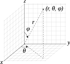
Suppose we have a vector $\vec{S} = \{S_x, S_y, S_z\}$ and suppose we want to give a Hamiltonian description to its direction. The phase space we want to consider, then, is the space of all possible directions, which we can think of as the sphere of unitary radius. The norm of the vector $|\vec{S}|$, instead, is a parameter for the system, much in the same way that mass is a parameter for a massive particle. So, for convenience, we will assume that $\vec{S}$ is unitary.
The first order of business is to find a set of conjugate variables. Recall that $x$ and $p_x$ are conjugate because the area $dx \wedge dp_x$ does not change under coordinate (i.e. unit) transformations. Note that the solid angle $d\Omega$ is already a quantity that is independent of coordinates so, using spherical coordinates, we can write:
\begin{equation}
\begin{aligned}
d\Omega &= \sin \varphi d\varphi d\theta \\
&= – d(\cos \varphi ) d\theta \\
&= – d(\cos \varphi ) \wedge d\theta \\
&= d\theta \wedge d(\cos \varphi )
\end{aligned}
\label{DirectionDOF}
\end{equation}
The minus sign is removed since the wedge product is anti-symmetric (i.e. $a \wedge b = – b \wedge a$). Note that $\cos \varphi $ is the component of the vector along the vertical direction. So our conjugate variables are $\theta^{xy}$, the angle on the $(x, y)$ plane, and $S_z$, the vertical component.
In terms of the conjugate variable, we have:
\begin{equation}
\begin{aligned}
S_x &= \cos \theta^{xy} \sqrt{1-S_z^2} \\
S_y &= \sin \theta^{xy} \sqrt{1-S_z^2} \\
S_z &= S_z\\
\end{aligned}
\label{SpinComponents}
\end{equation}
We can calculate the Poisson brackets:
\begin{equation}
\begin{aligned}
\{S_x, S_y\} &= \frac{\partial S_x}{\partial \theta^{xy}}\frac{\partial S_y}{\partial S_z} – \frac{\partial S_y}{\partial \theta^{xy}}\frac{\partial S_x}{\partial S_z} \\
&= -\sin \theta^{xy} \sqrt{1-S_z^2} \sin \theta^{xy} (- \frac{S_z}{\sqrt{1-S_z^2}}) \\
&\; – \cos \theta^{xy} \sqrt{1-S_z^2} \cos \theta^{xy} (- \frac{S_z}{\sqrt{1-S_z^2}}) \\
&= \sin^2 \theta^{xy} S_z +\cos^2 \theta^{xy} S_z \\
&= S_z \\
\{S_y, S_z\} &= \frac{\partial S_y}{\partial \theta^{xy}}\frac{\partial S_z}{\partial S_z} – \frac{\partial S_z}{\partial \theta^{xy}}\frac{\partial S_y}{\partial S_z} \\
&= \cos \theta^{xy} \sqrt{1-S_z^2} \cdot 1 – 0 \\
&= S_x \\
\{S_z, S_x\} &= \frac{\partial S_z}{\partial \theta^{xy}}\frac{\partial S_x}{\partial S_z} – \frac{\partial S_x}{\partial \theta^{xy}}\frac{\partial S_z}{\partial S_z} \\
&= 0 – (-\sin \theta^{xy} \sqrt{1-S_z^2}) \cdot 1 \\
&= S_y \\
\end{aligned}
\label{SpinBrackets}
\end{equation}
Note that these are analogous to the same relationships one has with spin components and commutators in quantum mechanics.
2. Relation to spin and magnetic field
Suppose we have the following Hamiltonian $H=\mu\vec{B}\cdot\vec{S}=\mu B^i S_i$, which is formally identical to the Hamiltonian for a spin 1/2 system in a uniform magnetic field. We can calculate the evolution of the vector components using the standard Hamiltonian techniques. For simplicity, let’s assume our “field” $\vec{B}$ is oriented along the $z$ axis, that is $H= \mu B^z S_z$. We have:
\begin{equation}
\begin{aligned}
\frac{dS_x}{dt} &= \{S_x, H\} = \mu B^z \{S_x, S_z\} = – \mu B^z S_y \\
\frac{dS_y}{dt} &= \{S_y, H\} = \mu B^z \{S_y, S_z\} = \mu B^z S_x \\
\frac{dS_z}{dt} &= \{S_z, H\} = \mu B^z \{S_z, S_z\} = 0 \\
\end{aligned}
\label{SpinEquations}
\end{equation}
Integrating, we have:
\begin{equation}
\begin{aligned}
S_x &= S^0_x \cos \omega t – S^0_y \sin \omega t \\
S_y &= S^0_x \sin \omega t + S^0_y \cos \omega t \\
S_z &= S^0_z \\
\omega &= \mu B^z
\end{aligned}
\label{SpinPrecession}
\end{equation}
The vector $\vec{S}$ precesses about the axis determined by $\vec{B}$, and in the plane orthogonal to it, with angular velocity $\mu B^z$. This is exactly what spin does in a magnetic field.
As we have seen, we can construct a classical analogue of spin just by looking at the Hamiltonian evolution of spatial directions. Like in the case of position and momentum, we have two conjugate variables and we have the same set of relationships and equations between them.
Another thing to note. In Hamiltonian mechanics the conjugate variables are a pair. If the spatial direction is an independent degree of freedom then it must be described by a pair of variables. Note that a direction in an $n$ dimensional space is always described by a set of $n-1$ variables. Therefore the only direction we can describe in Hamiltonian mechanics as an independent degree of freedom is a direction in a three dimensional space since we must have $n-1 = 2$.